Since I caught the financial independence bug a short 6 months ago, I have been fired up about pinpointing how I can contribute to the community. It is my dream to help others strive for mental and financial freedom by challenging their thinking, taking action, and pursuing their own aspirations. I aim to merge this vision with my data modeling and visualization skills to build capabilities that empower others to make informed decisions.
My first blog post will focus on a tool I built that presents a framework for how to approach the age-old question to rent or buy your primary property. This first model turned out to be a bit more intricate than I originally envisioned. Those that know me won’t be surprised by this, but I will strive to make smaller, bite-sized tools in the future.
I don’t want to create these tools in a black hole. I want to hear your feedback and ideas. Please consider leaving a comment or reaching out directly so we can work together and make a greater impact.
Disclaimer & Scope
I am enrolled in a CFP® Certification Professional Education Program, but I do not currently hold financial licenses or certifications. I’m making this model available to spur conversation and gather feedback. I make no promises, implied or otherwise, by sharing this tool. This tool is for experimentation and should not be used in isolation to make such an important decision. It does not provide any type of advice.
Setting the Stage: Decision Factors
There are numerous personal factors that play into the decision to rent or buy. Perhaps the most glaring is your desired lifestyle, but there are a plethora of additional elements to consider. Some are more difficult to quantify than others. There are general guidelines to consider, like the 5-year rule stating that you are more likely to earn a profit if you live in the property for at least 5 years before selling. This timeline reduces the likelihood that earned equity and appreciation will be washed out by homeownership expenses and closing costs. The price-to-rent ratio is another common guide that provides rough guidance to determine which decision makes more sense on paper based on market trends. While rules of thumb tend to be directionally accurate, they are generalizations. They are inflexible and do not account for variables unique to your situation.
Considering housing tends to be one of the largest structural expenses in our budgets, I wanted to develop a capability that accounts for individuals’ unique situations, making the decision more personal. I also desired to create a method to define and quantify opportunity costs. I find that evaluating alternatives up front tends to lead to greater peace of mind with whatever outcome prevails. It also serves as a thought exercise to consider the variables you are optimizing; they may extend beyond money.
Assumptions
The tool:
Assumes you invest any difference between the cost of buying vs. renting in low-cost index funds. Therefore, if rent is $2,500/month, and a mortgage payment and other home-associated costs total $3,500/month, it assumes you invest the entire expense difference of $1,000 that month. It does not account for what you may do with any additional income. Rather, it highlights the opportunity cost of the difference in expense between renting and buying.
Does not currently account for variable interest rate loans due to the unpredictable nature of rates and the fact that we’re focusing on averages over longer time horizons.
Is intended to help individuals considering their own primary housing situation. It does not account for special situations like live-in-landlords who receive income from tenants or traditional rental properties. I am planning to build separate decision-support tools for those cases once I receive feedback from the community.
Does not consider the future value (FV) of funds accounting for inflation; funds are based on the purchase year specified in the data entry tab.
Does not account for variability in home price appreciation. Rather, it currently implements a fixed average return in the Data Entry tab. This is one of the reasons the Monte Carlo Simulation results for the buy scenario have less variability than the rent scenario. I may update if it is requested.
These elements were not included in this iteration by design to eliminate as many secondary factors as possible and isolate the “Rent vs. Buy” decision. For example, including factors like savings rate, which will vary from person-to-person, removes emphasis from the decision to rent or buy.
To assess whether renting or buying is right for you, it is necessary to identify costs and related variables relevant to each decision. This is the purpose of the Data Entry tab. Once you enter your data (or other data of interest), the tool will update throughout and you may engage in “what-if” analyses by changing values based on personalized factors. No data input is allowed in any other tabs in the workbook. Only cells in blue may be modified – others are locked as they will automatically update based on your inputs in blue cells.
For additional utililty, I incorporated tables that account for variables like additional mortgage principal payments and unplanned (non-routine) maintanence expenses. You may also run scenarios to determine how changes in rate variabes, like expected market return and increases in rental costs, may alter potential outcomes.
All tables are formatted as Excel data tables. Therefore, if you add a row to an existing table, calculations that reference the table will automatically update to include new records. I encourge you to experiment with various variables to see how they may influence your decisions.
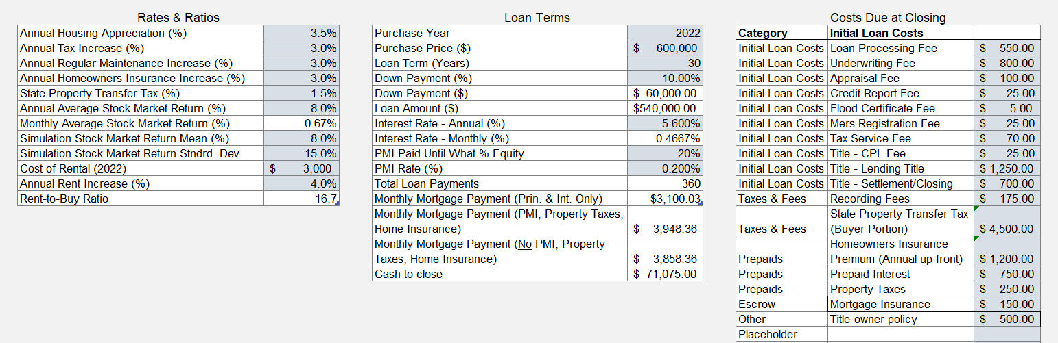
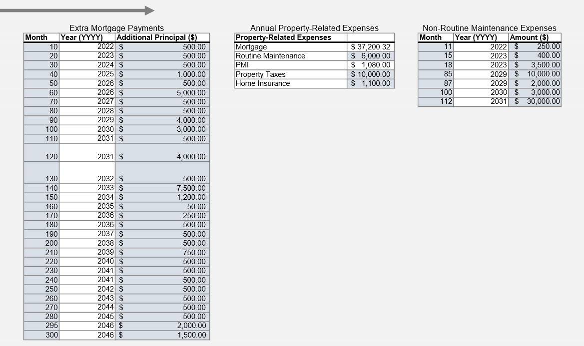
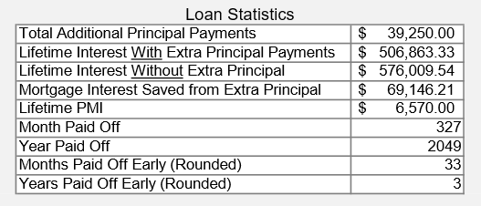
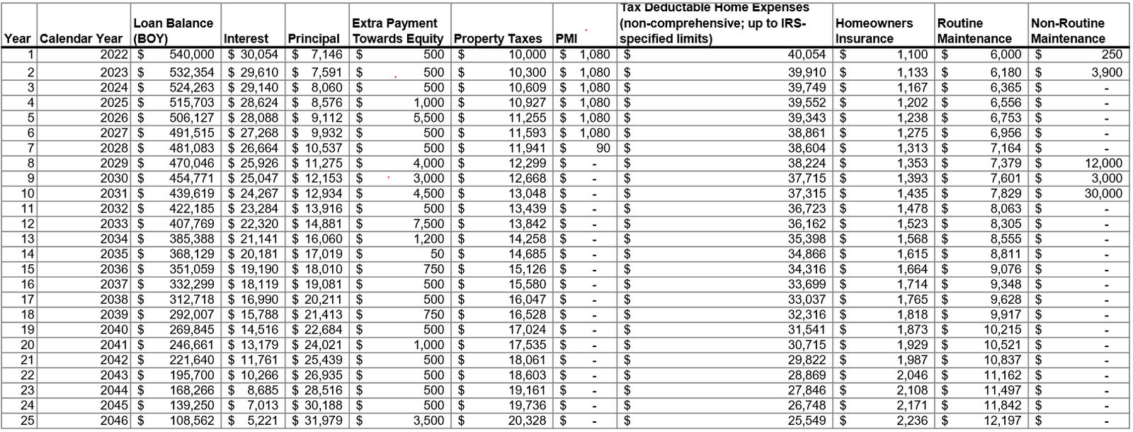
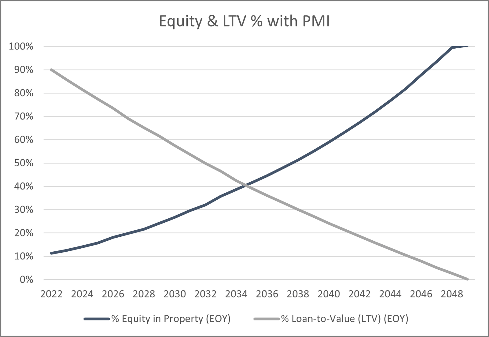
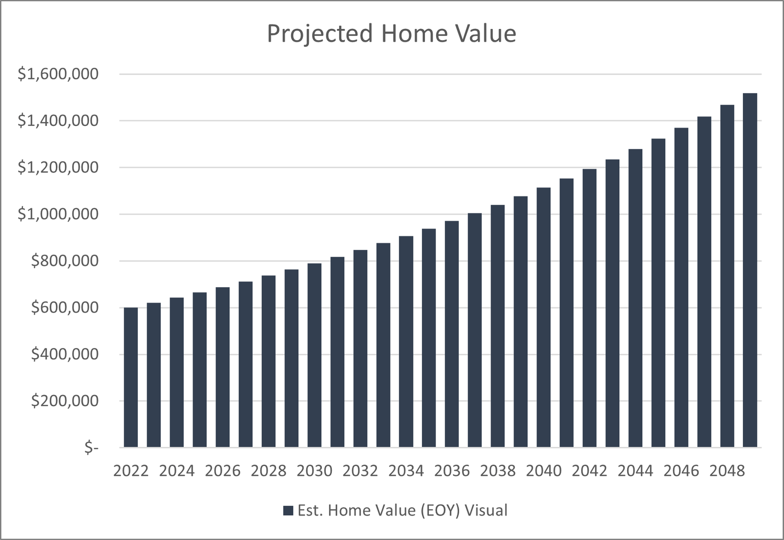
From left to right, the first three tables, pictured in Figure 1, capture baseline prices/figures and their anticipated rates of increase (e.g., home appreciation, tax, rental increases), loan terms, and closing costs. Tables 4-6 , presented in Figure 2, provide an opportunity to enter any additional mortgage principal payments you plan to make (or have already made), annual property-related expenses (routine), and unplanned (non-routine) maintenance expenses. Figure 3 provides summary loan statistics like PMI and interest paid, comparing total interest paid with and without extra principal payments.
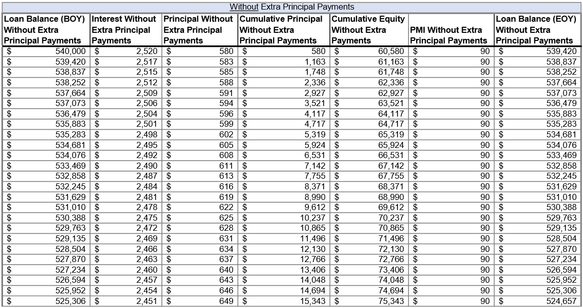
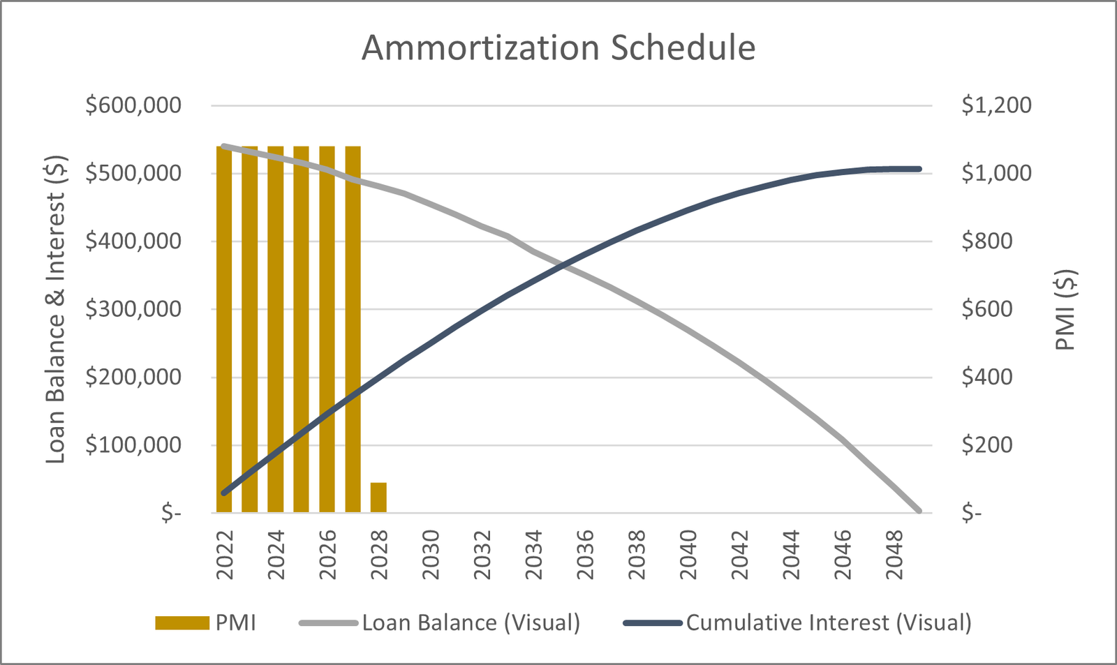
Monthly Mortgage Ammortization Tab
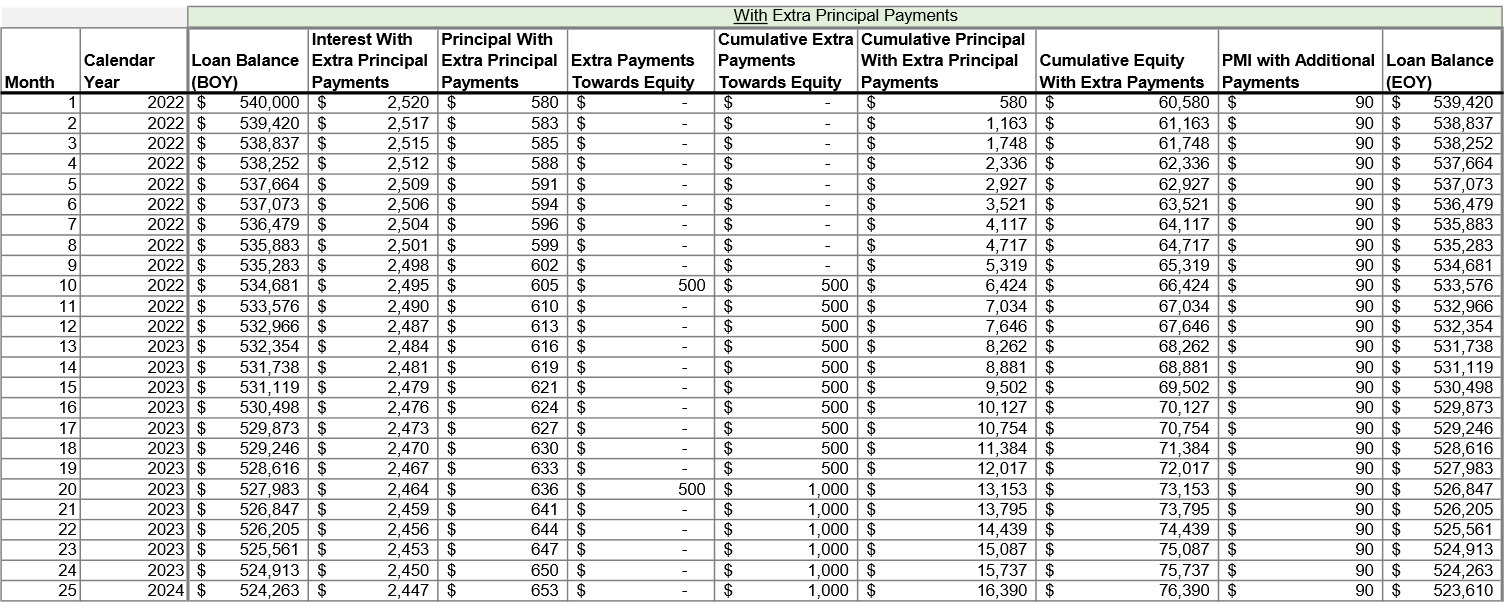
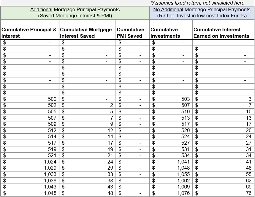
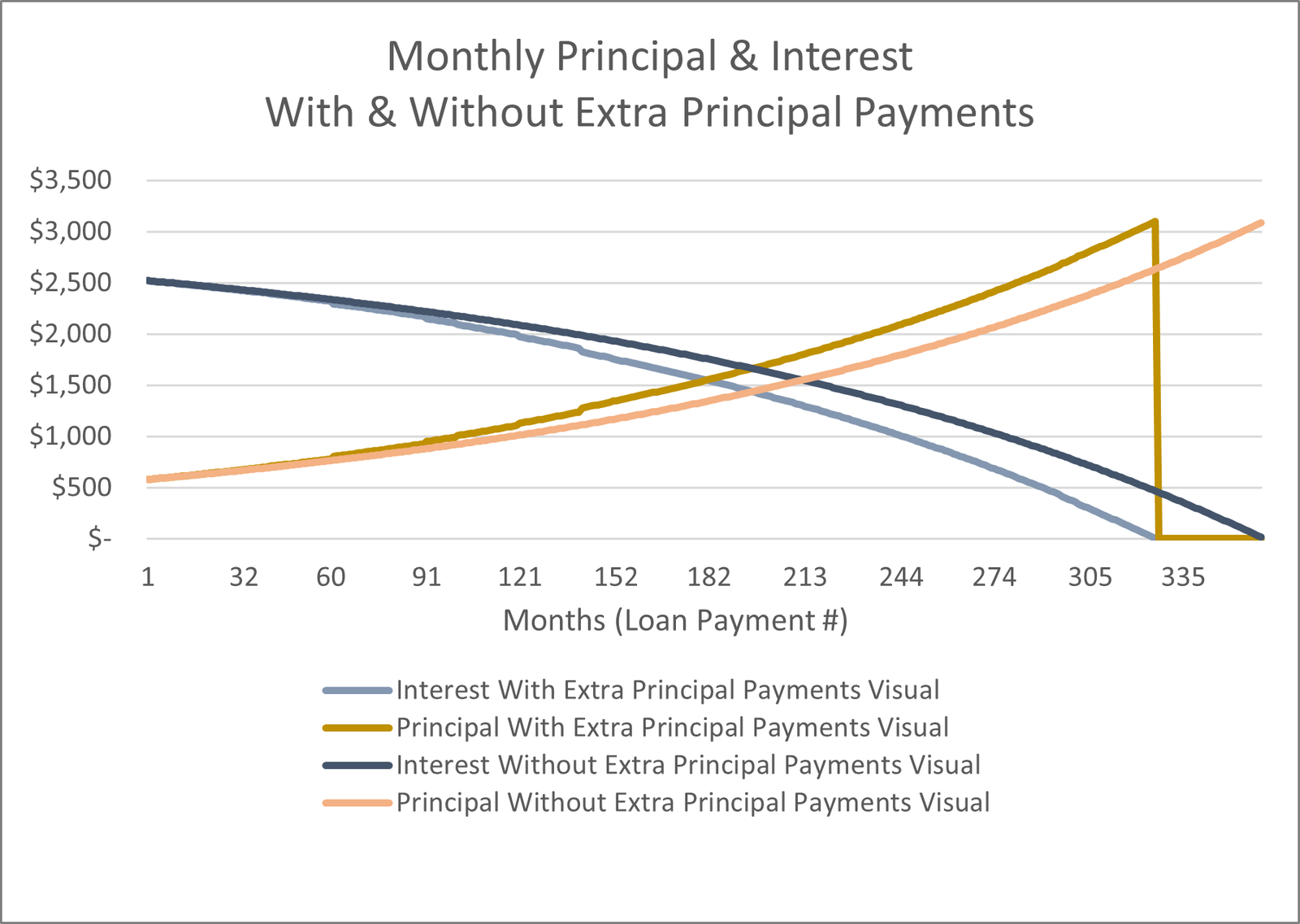
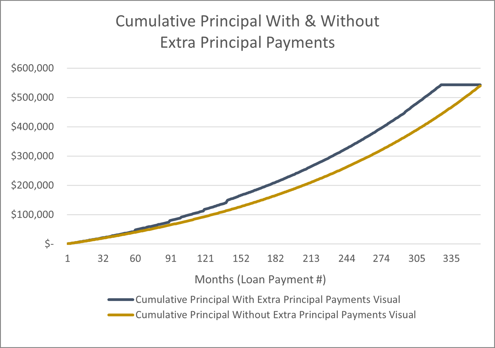
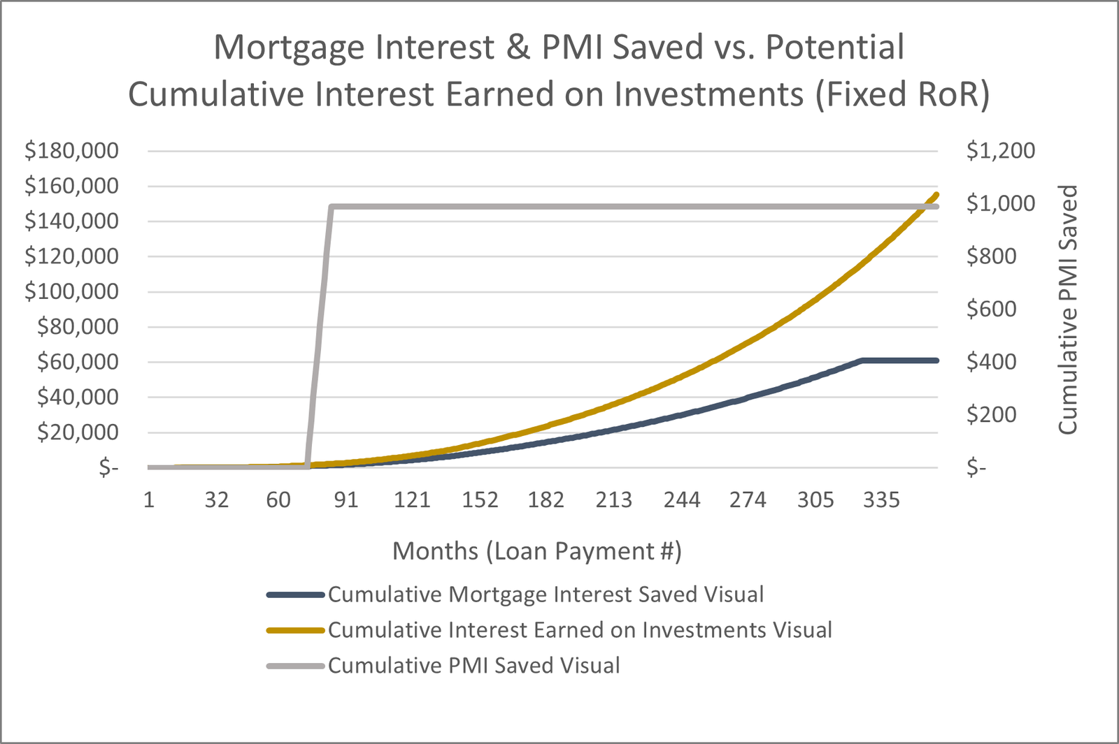
The next tab, a monthly mortgage amortization schedule, contains two versions: the first includes additional payments towards principal (Figure 4), whereas the second does not (Figure 5). This provides a method to quantify the value of extra payments. Of course, making extra payments introduces an opportunity cost of those funds. To account for this, we calculate mortgage interest and PMI saved with extra payments and compare it to potential interest/earnings if the money was invested in low-cost index funds (assuming fixed RoR in this case). Figure 6 contains this comparision.
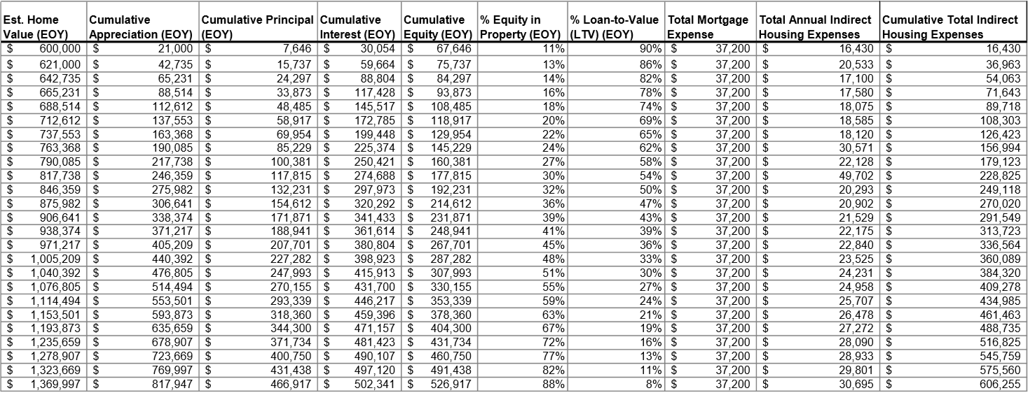
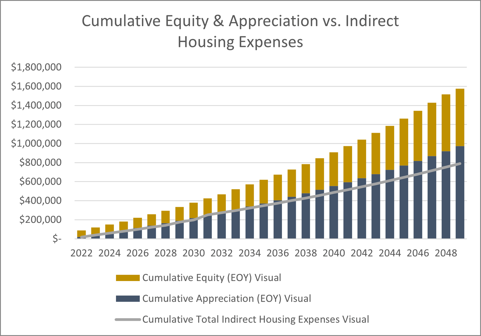
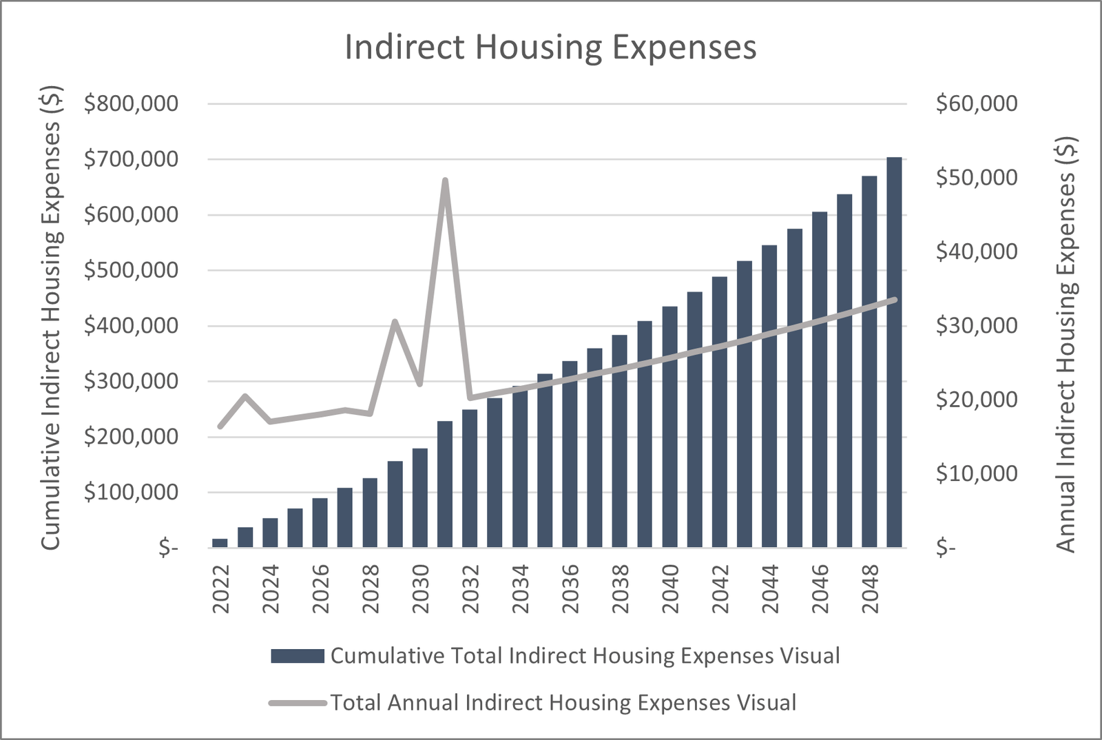
We then roll the monthly data into an annual mortgage amortization schedule, reflected in Figures 10-11, and incorporate other home-related expenses, like maintenance and property taxes. Cumulative figures like appreciation and equity are also included here, which tend to be more intuitive in an annual schedule.
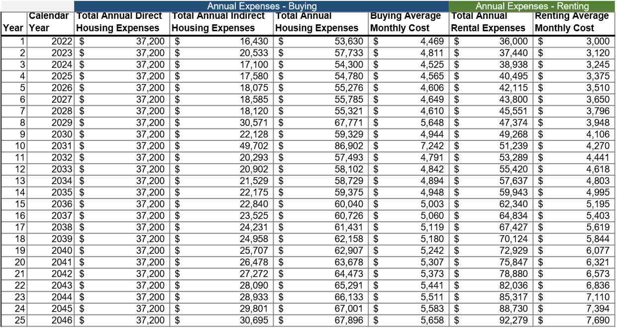
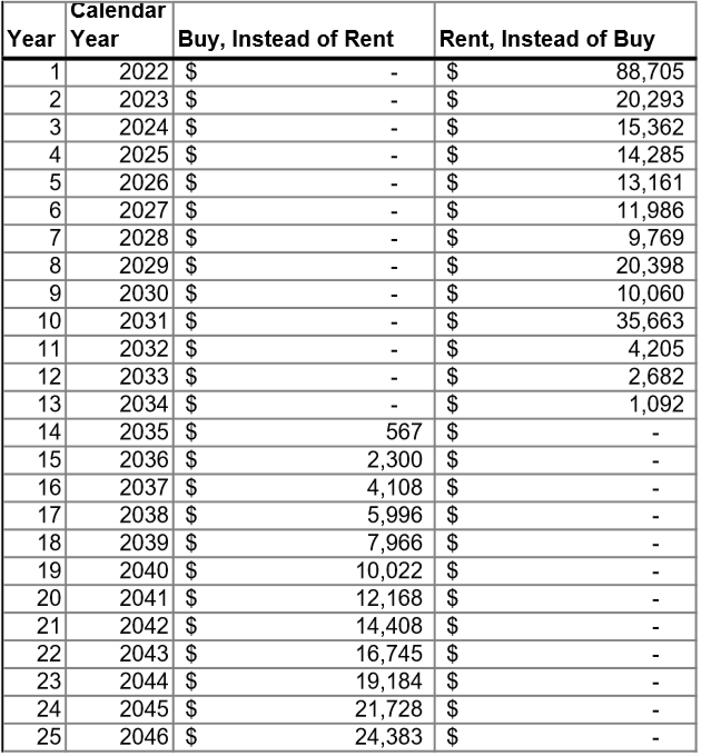
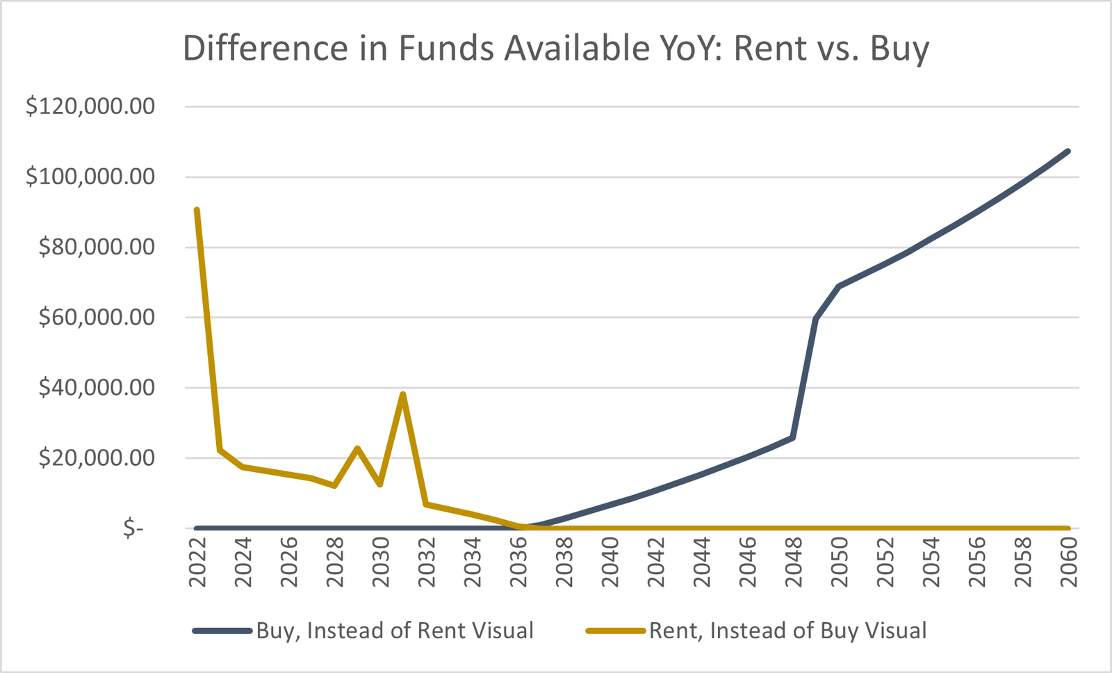
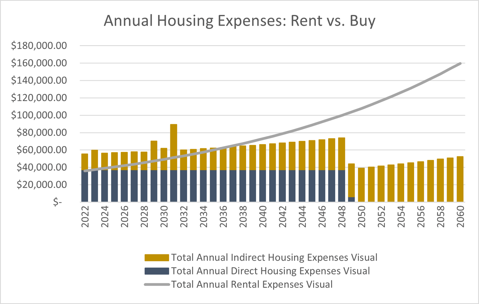
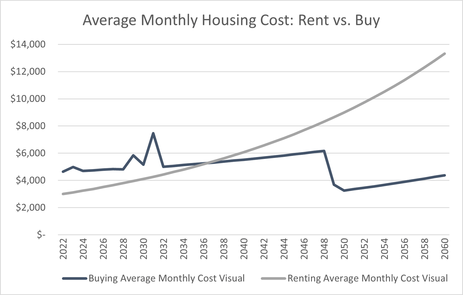
Now that we have pinpointed mortgage-related costs by implementing ammoritzation schedules and related expenses, we may now compare overall projected expenses for both rent and buy scenarios. Figure 17 captures direct and indirect housing expenses, in addition to total rental costs. Figure 18 illustrates the difference between total expenses for each case. This reveals the estimated opportunity cost, in dollars, of each decision.
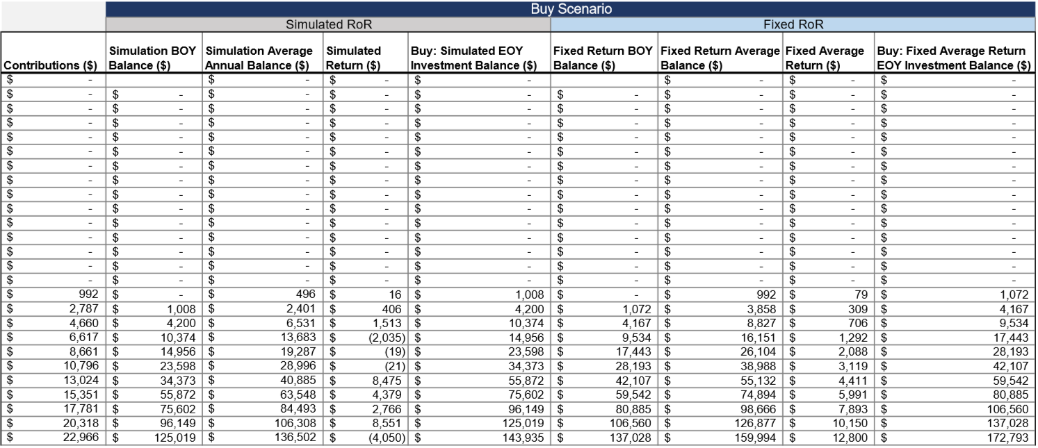
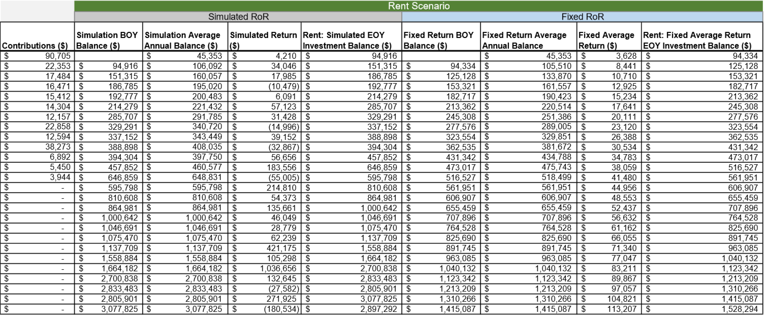
After considering the difference in expenses, we must also consider how we will put that money to work for us. That’s where investments come in. For each scenario, renting and buying, we assume that we will invest the entire difference of funds available in low-cost index funds. If we buy, we lose the ability to invest that money in low-cost index funds up front, but we benefit from immediate property appreciation and equity growth. If we rent, we may invest the initial closing costs that would otherwise be consumed by the house, but we don’t have ownership of an appreciating (hopefully) asset.
As mentioned, we assume we invest the difference between mortgage costs and rent. For example, in year 1, if closing costs are $60,000 and the mortgage is $3,500/month, while rent would cost $2,500/month, we assume the individual would invest a total of $72,000 ($60,000 + ([3,500-2,500]*12).
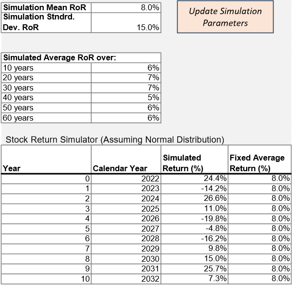
For both rent and buy scenarios, we provide both simulated and fixed RoR projections to compare potential outcomes. Simulated returns are estimated using a normal distribution. While a normal distribution doesn’t account for extreme events as well as, say, a t-distribution (with fatter tails to account for rare, but highly-impactful market events), it is used here for simplicity. We are also assuming a medium to long-term investing strategy, which would provide time to recover from extreme events with time.
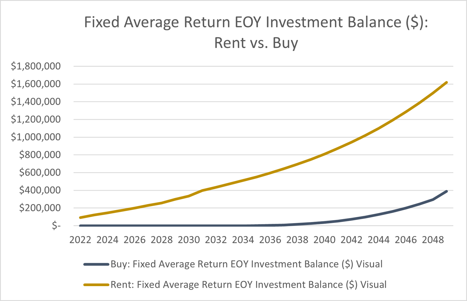
If you’re asking why buying looks like such a poor option in Figures 25-26, you’re on the right track. It is because they only represent the invested balance of funds, and don’t account for the cumulative equity or appreciation that result from owning a home.
Projected Assets Tab
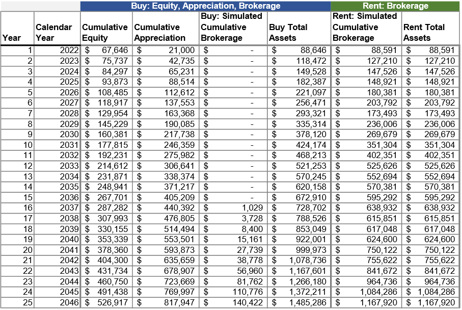
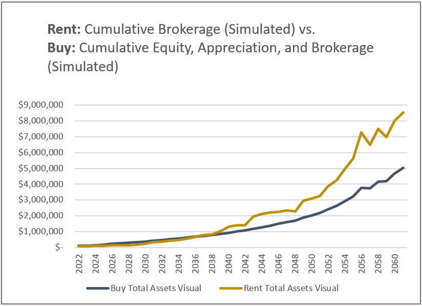
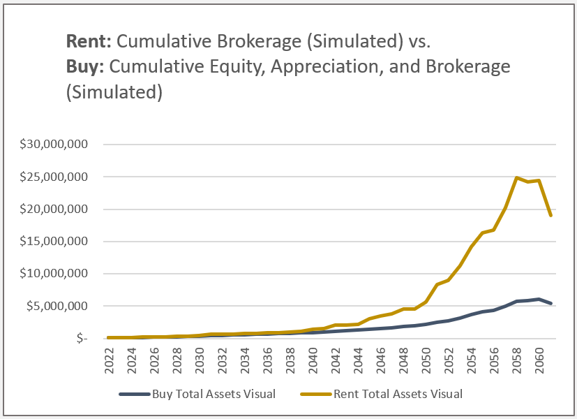
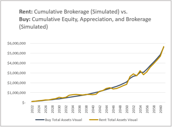
To make this a fair comparison, we next compare total assets. If you rent, you will theoretically only have the funds that you’ve invested. If you buy, you will have the funds you invested, cumulative equity (down payment and principal) and appreciation. Figure 27 accounts for total assets in each scenario.
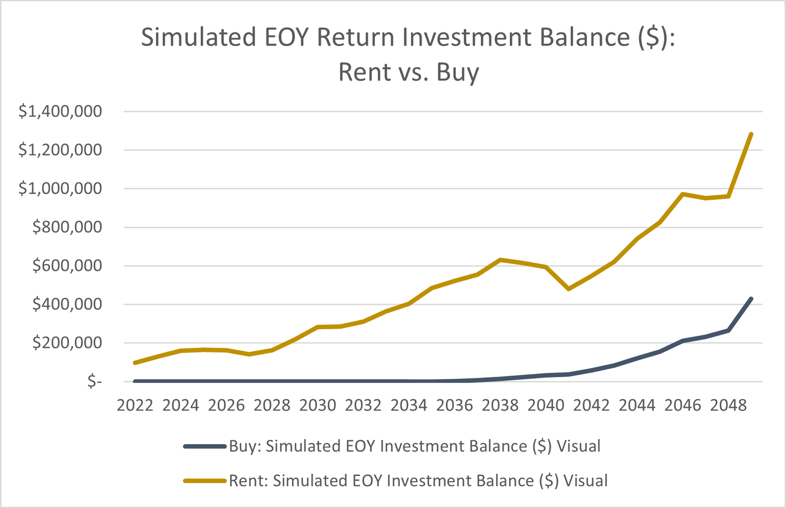
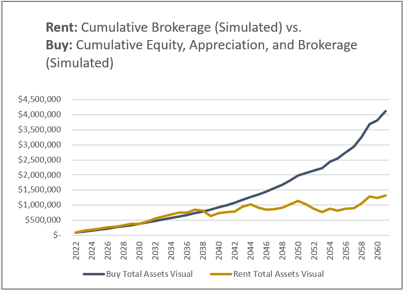
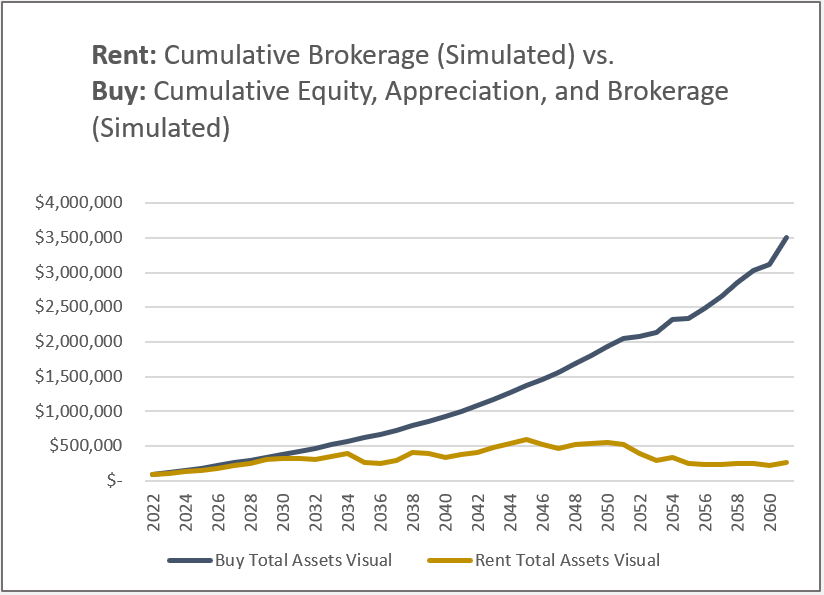
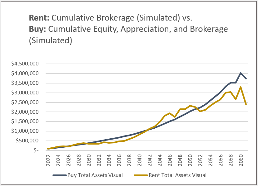
Figures 28 – 33 below represent 6 seperate simuation runs, each representing total assets in Rent and Buy scenarios. You may run your own simulation trials, which alter only the expected investment returns, by navigating to the “Formulas” tab and selecting “Calculate Now” in the top right.
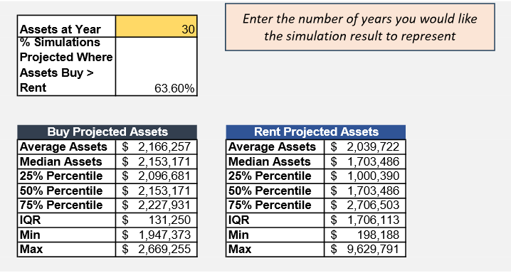
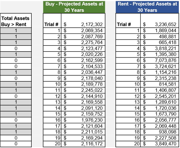
While we may manually run simulations as described above, I incorporated a Monte Carlo analysis to capture averages over larger volumes of simulation trials. I limited the simuation to just 250 trials at this point due to my personal machine processing limitations, but will expand this in the future to produce more robust results. Figure 37 displays the first 20 trial run results with a running tally of which scenario led to a higher total assets value for each trial.
You will note that in Figure 36 there is an option to enter a numeric value in the “Assets at Year” row. The default is 30 years, but this may be changed to your value of choice to represent outcomes at difference points in time in the future. As we saw, buying tends to be associated with higher initial expenses than renting; however, as rent increases, mortgage costs are more stable than rent. The field below represents the % of simulations where assets in the buy scenario were higher than those in the rent scenario. Additional statistics based on simulation results are included, also.
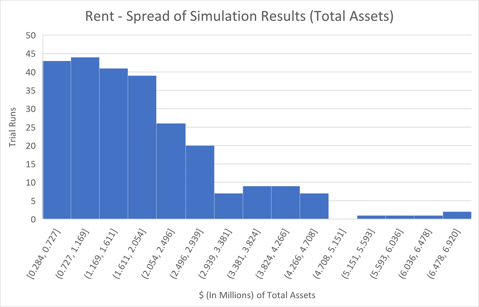
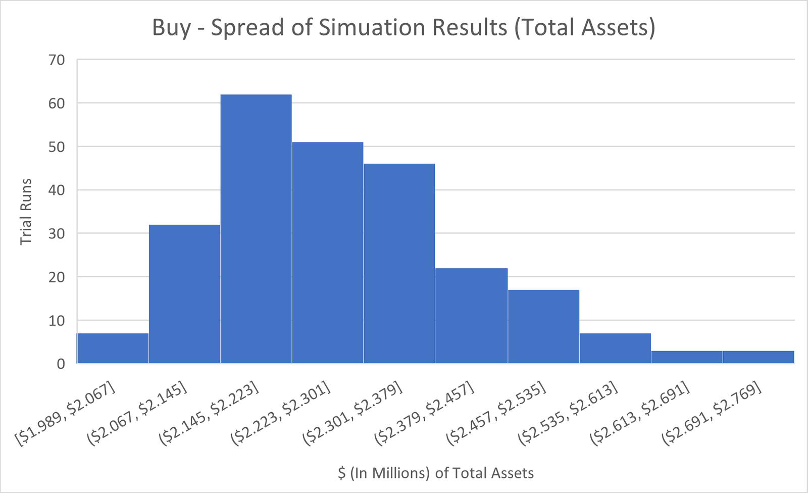
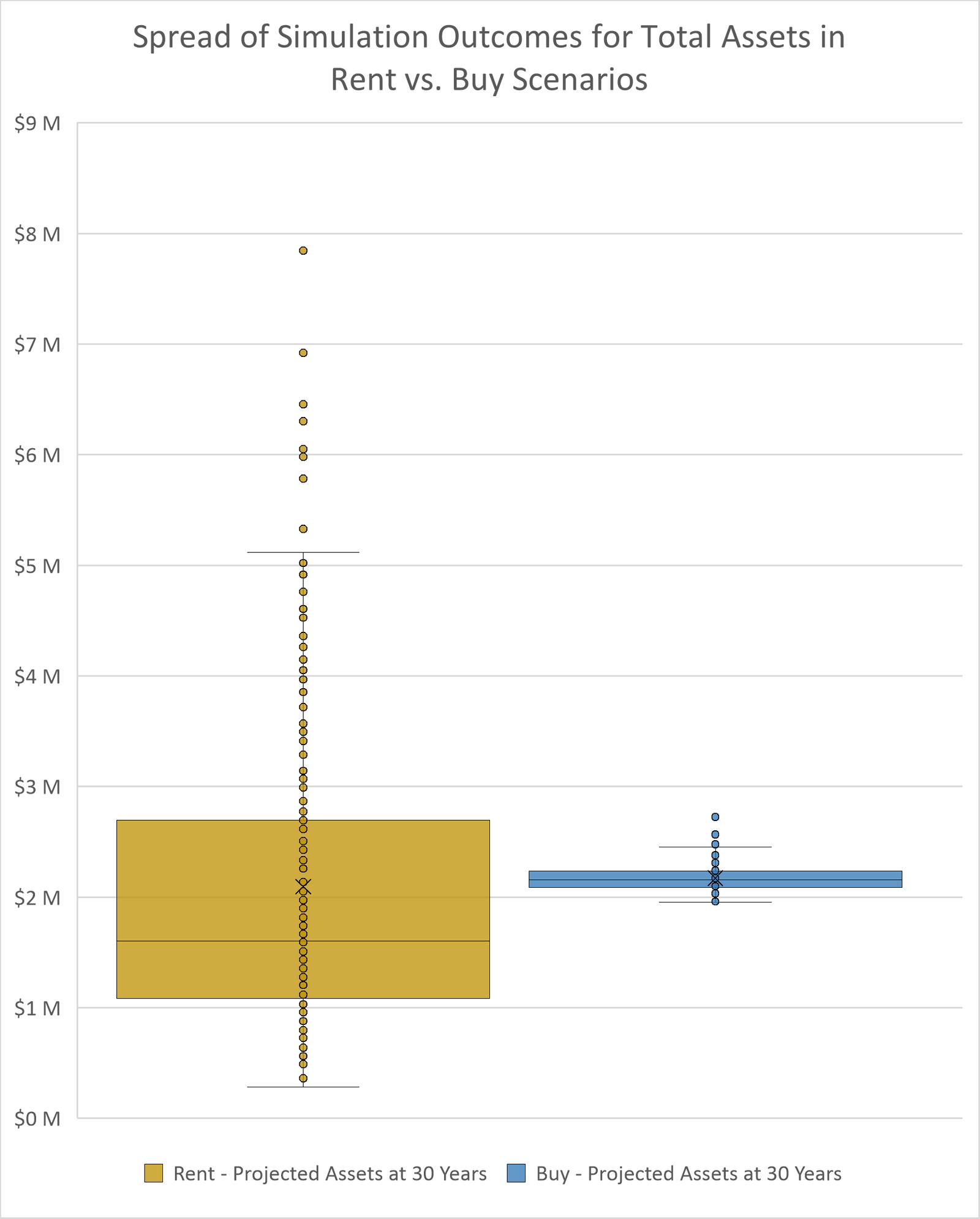
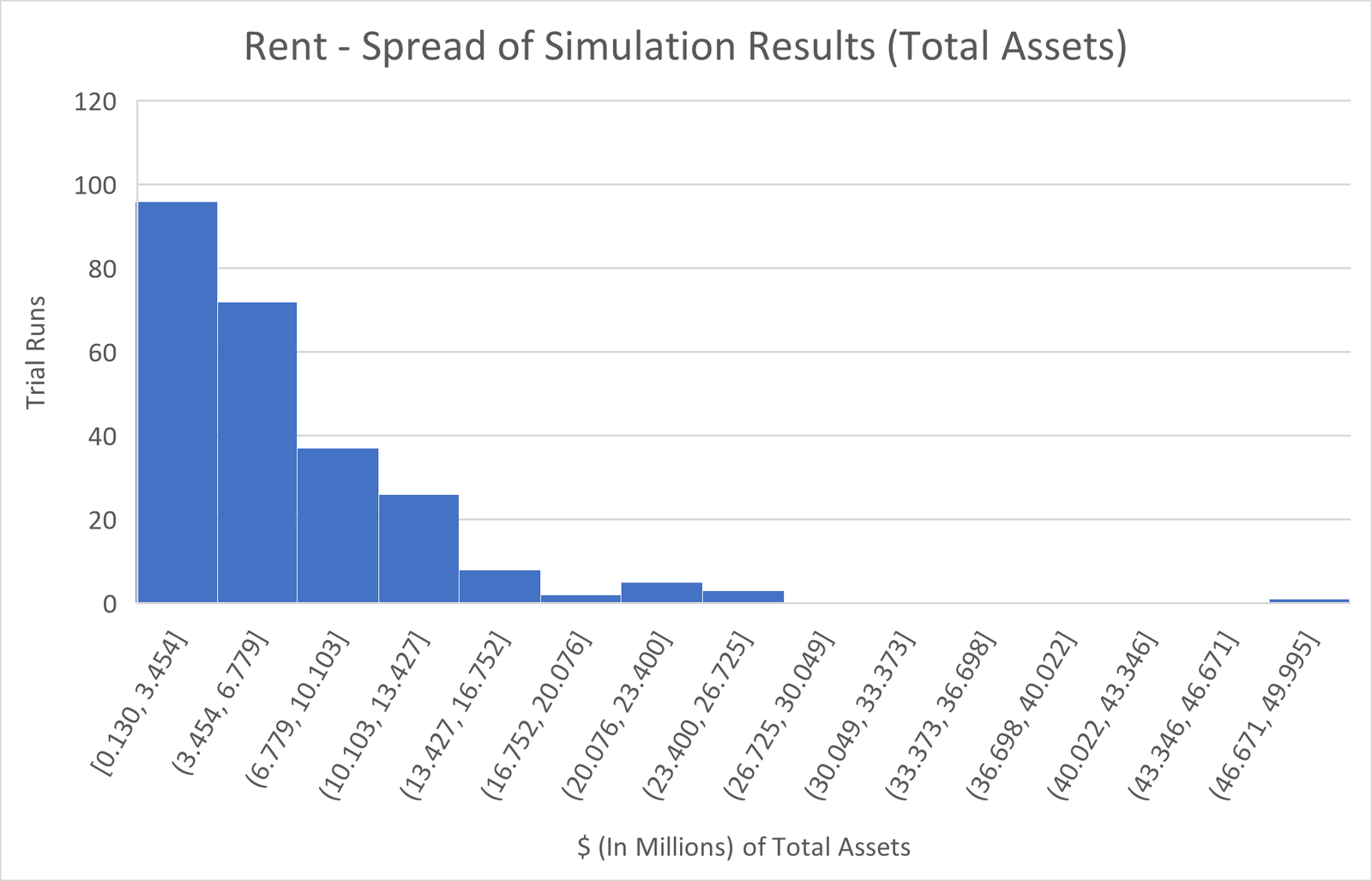
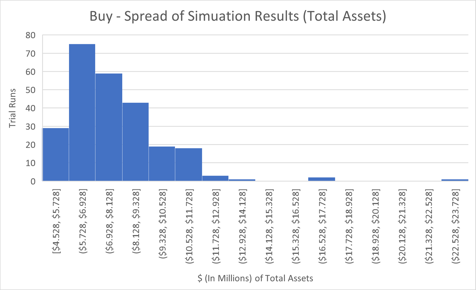
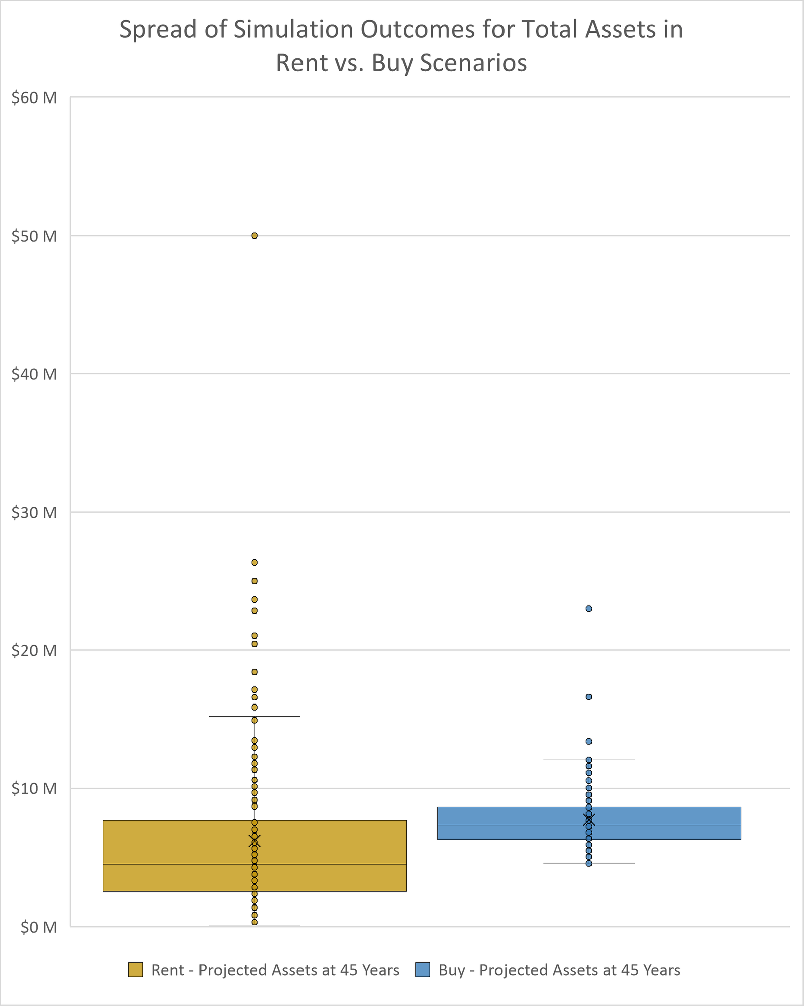
I then built histograms for both rent and buy scenarios referencing the results of the Monte Carlo Simulation to display the spread of possible outcomes. Notice how the buy scenario results in a distribution with a slight right skew, whereas, the rent scenario produces a significantly heavier right tail. This is expected since the renting scenario only accounts for low-cost index fund investments. Finally, Figure 40 contains a box-and-whisker plot to better compare the distribution of trial outcomes side-by-side.
Due to the higher allocation of index funds that make up total assets when renting when compared to buying (with the default parameters – your case may be different), it is not surprising to see the greater spread of expected returns in the rental scenario. While you may realize a greater return, that return is perhaps more volatile. On the flip side, the buying scenario has a much lower expected deviation from the mean total assets, but no trial runs resulted in total assets exceeding $3M when evaluated at 30 years in the future.
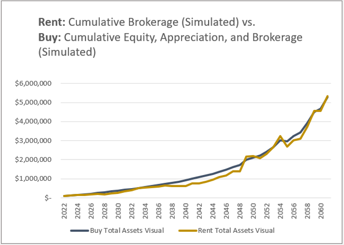
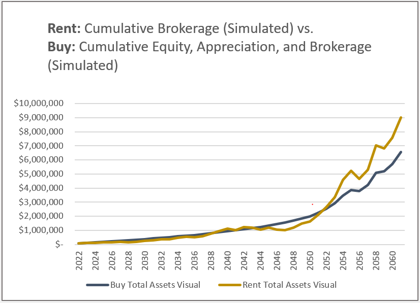
However, once we evaluate the model further in the future, say 45 years, the results begin to transform. See Figure 41.
Notice how total assets in the buy scenario begin to pull ahead relative to the rental scenario when comparing T+30 to T+45 years. Of course, this will depend heavily on the variables you enter in the Data Entry tab, which is why I encourage exploration.
Conclusion
Ultimately, there is no ‘right’ answer. In addition to the financial variables discussed, there are many non-financial factors to consider while making the decision to rent or buy. We will discuss those another time, but my hope is that this model provides a strong framework for how to quantify the financial variables at play to guide the Rent vs. Buy decision.
Please leave a comment and provide your feedback. I would love to hear from you as I begin my blogging journey and continue to share tools that support decision making and raise awareness of critical financial topics. Thank you!